Configuring DIMENSION4

The Location System Config tool (LSC) allows you to configure your D4 RTLS to locate tags in real-time, which involves:

• Setting up logging servers to store the generated data.

• Importing background representations and objects to create a 3D environment of your physical location tracking space.
• Adding and configuring devices including UWB Sensors (sensors), Timing Distribution Units (TDUs), and 2.4GHz Receivers.
• Solving sensor parameters to generate accurate sightings of tags.
• Setting up tag filters.

The LSC contains various tabs that are listed in the order in which you are likely to complete these tasks.

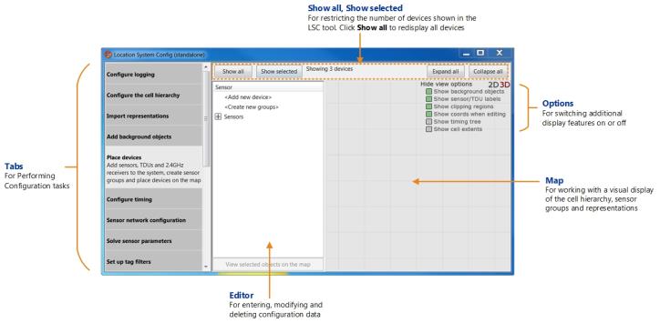
Location System Config User Interface

Configuring Logging

The D4 RTLS generates large amounts of log data, including:

• Event data (tag location information captured by sensors).

• Trace messages about the performance of your D4 RTLS.

For audit and optimization purposes, we recommend that you capture and store log data according to your business policies.

To set up logging:

1. Identify the logging requirements of your D4 RTLS.

2. Determine how to structure your logging system.

3. Configure logging servers, and then assign them to various cells. For information about cells, see Configuring the Cell Hierarchy.

Adding a Logging Server

Before you add a logging server, ensure that:

• A suitably configured Location Platform is installed on the server

• The logging server has sufficient disk space to store log messages

  To determine the required disk space for logging, use the spreadsheet LoggingDiskRequirements.xlsx. The spreadsheet allows you to calculate the required disk space based on the number of tags, tag update rate, and other parameters.

Additional information on configuring logging is provided in Setting up DIMENSION4 logging at a production site .

To add a logging server:

1. On the Configure logging tab, in the lower pane, double-click <Add server log properties>.

2. Select the server that you want to add.

3. Set the maximum disk space (in MB) to use on the server.

4. Set the path to the log directory to use on the server.

5. Click Save.

The logging server is added. You can now assign it to various cells.

Assigning a Logging Server

When you assign a logging server, it is inherited through the cell hierarchy:

• The logging server of the Site Cell is inherited by its Geometry Cells and Location Cells.

• The logging server of a Geometry Cell is inherited by its Location Cells.

You can also assign separate logging servers to the Site Cell and each Location Cell.

Assigning a Logging Server to a Cell

To assign a logging server:

1. On the Configure logging tab, in the upper pane, expand the cell hierarchy. The cell hierarchy shows the existing Site Cell, Geometry Cells, and Location Cells.

   If a cell does not have a logging server assigned, the cell status appears as <logging disabled>.

2. To assign a logging server, click to select the cell and then slowly double-click <logging disabled>, or press the Enter key.

   The <logging disabled> status changes to a drop-down list.

3. From the list of available servers, select the logging server that you want to assign.

Inheriting a Logging Server

If you have assigned separate logging servers to various cells, but want to inherit the logging server from a parent cell:

1. Select the cell.
2. From the Server drop-down list, select <inherit server from parent>.

Retrieving Log Data

The log data primarily captures:

• Tag locations, tracked by the sensors.
• Trace messages about the performance of your D4 RTLS.

To retrieve log data, use either the Review location events tab as described in Reviewing Location Events, or the View trace messages tab.

Changing Logging Server

You can change a logging server in the D4 RTLS at any time, for example:

• If you need to replace or upgrade the machine on which the logging server is running.

• If you delete a Location Cell, in which case you can optionally remove the log server properties for logging servers that are no longer used.

• If the logging destination, either the server or the server name, has changed.

To replace a logging server in LSC

1. Set up a new logging server as described in Adding a Logging Server.
2. If required, archive the logs for today and the previous 3 or 4 days; the number of days depends on your operating environment.
3. Assign the new logging server to the cell.

To remove a logging server from the D4 RTLS

1. On the Configure logging tab, select the server that you want to delete, and then press the Delete key.

   The server is removed from the list of logging servers.

2. If the server is assigned to one or more cells, reassign a different logging server to the cells, as required.

Configuring the Cell Hierarchy

Setting up a cell hierarchy involves defining the 3-dimensional space within which the tags will be tracked. A valid cell hierarchy contains three different types of cells that are listed in the following table.

Cell	Purpose
Site Cell	The Site Cell represents the entire site that is covered by the D4 RTLS. The Site Cell is created by default when you install the LSC.
Geometry Cell	The Site Cell contains one or more Geometry Cells. A Geometry Cell represents a smaller area within the Site Cell, such as: a floor of a building. a production area.
Location Cell	A Geometry Cell contains one or more Location Cells. A Location Cell represents a particular region or area where sensors are installed (sensor groups), such as: a process in a production area. a phase in the production cycle. any area where continuous tracking of tagged assets is required. In order to allow for continuous tracking of assets, make sure that Location Cells fully cover the areas where tags will be located.

In a valid cell hierarchy:

• All Geometry Cells are contained by the Site Cell.

• A Location Cell is contained by a unique Geometry Cell.

• The Location Cells do not overlap.

Tags are tracked as they move into and out of the areas where sensors are installed. Event information is recorded for each Location Cell and passed up the cell hierarchy, from each Location Cell up to the Site Cell.

Creating a Geometry Cell

To create a Geometry Cell:

1. Click the Configure the cell hierarchy tab.

2. Create a new Geometry Cell by following the onscreen instructions. Using your mouse, add points to create the required extent for the cell – it must cover the area of interest. When you click and drag to add a point, the coordinates of the point are displayed.

   Notes:

   • When defining the cell extent, you may prefer to work in the 2D view.

   • The Geometry Cell can be any shape. However, we recommend that you create a cell that is reasonably square or rectangular, and that you avoid a long, thin rectangle.

   • If there are multiple Geometry Cells, ensure that they do not overlap.

3. Define the top and bottom boundaries of the Geometry Cell to contain the Location Cells (and Sensor Groups).

   Field	Description
   Top	The height of the cell in meters. Any heights set for the Location Cells (or the Sensor Groups) contained by this Geometry Cell must be equal to or less than this value.
   Bottom	The floor height of the cell in meters. Any floor heights set for Location Cells (or the Sensor Groups) contained by this Geometry Cell must be equal to or greater than this floor height.
   Snap Grid	Snaps the cell extent to the nearest intersection of lines in the grid, when you drag the points with your mouse.

4. After you have created the cell, you can use the View options to check it in either 2D or 3D.

5. Click Save.

When you create the Geometry Cell, it will not usually be inside the Site Cell. Follow the onscreen instructions in the Errors panel to fix this. The LSC tool automatically fixes the error by enlarging the Site Cell to contain the cell hierarchy.

Creating a Location Cell

To create a Location Cell:

1. Click the Configure the cell hierarchy tab and expand the Geometry Cell that will contain the new Location Cell.

2. Create a new Location Cell by following the onscreen instructions.

   Notes:

   • Place the Location Cell extent within a Geometry Cell.

   • The Location Cell can be any shape.

   • If there are multiple Location Cells, ensure that they do not overlap.

3. Define the top and bottom boundaries of the cell, ensuring that the Location Cell is contained within the Geometry Cell.

4. Save the cell. If there are any errors, the LSC tool displays messages to identify particular problems, and provides options to fix them.

After you have created a cell, you can check it in either 2D or 3D.

Starting Cell Services

Deploy the cell services for the Site Cell, each Geometry Cell, and each Location Cell:

1. Start the Service Manager tool. The Cells option lists all the Site Cells, Geometry Cells, and Location Cells that you have created.

2. You can deploy services for either:

   • The entire Site Cell, including all the Geometry Cells and Location Cells that it contains.

   • A particular Geometry Cell or Location Cell.

   After you deploy services for a cell, the status of the cell changes to Running.

Modifying a Geometry or Location Cell

To modify an existing Geometry or Location Cell:

1. On the Configure the cell hierarchy tab, double-click the cell to display the editor.
2. Modify the shape and/or extent of the cell, as required.
3. Click Save.

Deleting a Geometry or Location Cell

To delete a cell:

1. On the Configure the cell hierarchy tab, select the cell.
2. Press the Delete key.

• Geometry Cell: The Geometry Cell and its Location Cells are deleted.

• Location Cell: The Location Cell is deleted.

• Sensors, Sensor Groups and background objects are not deleted.

3. Using the Service Manager tool, undeploy services for the deleted cells:

   1. Go to Start > All Programs > Ubisense 3 > Service Manager 3.
   2. In the Cells & Controllers pane, open the Cells folder, and expand Site.
   3. Select the cell that you have deleted, and then click the Stop button.

Guidelines for Assembly Plants

When setting up a cell hierarchy for an assembly plant, ensure that you consider load balancing requirements. A few guidelines are as follows:

• Split a plant into Geometry Cells.

• If a production line is made up of parallel bands, ensure that a single band is covered by its own Location Cell.

• If a production line has a very long, continuous section, split the section into multiple Location Cells.

Importing Representations and Adding Background Objects

A representation is a 2D representation or 3D model, such as a map, floor plan, or objects in the physical location tracking environment. For example, you can use a map as a guide when placing sensors and TDUs.

Representations, such as a map, are optional. They are intended to help you with placing sensors. They do not affect the functionality of your D4 RTLS. However, if you want to use representations, you must size and scale them accurately.

Setting up a map and other background objects involves:

1. Importing a background representation and any other additional models that represent various objects from your physical environment.

2. Scaling (resizing) and modifying the alignment and position of each representation, as necessary.

3. Placing these objects as required.

Supported File Types

You can import the following file types:

• Bitmap (.bmp)

• COLLADA (.dae)

• Graphics Interchange Format (.gif)

• JPEG (.jpg and .jpeg)

• OpenSceneGraph (.osg)

• Portable Network Graphics (.png)

• Scalable Vector Graphics (.svg)

Importing Representations

Importing representations is optional. If required, you can import representations to:

• Provide a background, such as a floor plan, on which you can place other objects and sensors.

• Represent objects and items, which you can use as a guide when placing sensors.

To import a background representation and any other additional objects:

1. On the Import representations tab, import the images of the required background representations and objects.

2. Resize and reposition each representation as required, by modifying the following settings.

   To enter a value, click to select the row and then click again to make the box editable.

   Setting	Enables you to...
   Size and Scale	Resize the representation to the required measurements and scale. You can resize representations, including map representations, by using the Reference Points tool. See Transforming a Map Representation by Using Reference Points.
   Origin	Move the origin to the required position in the representation. For information on the importance of the origin for the background image, see Defining the Origin.
   Rotation	Adjust the orientation (in degrees) of the representation using the following options. Yaw: The horizontal angle of the image. Pitch: The vertical angle of the image. Roll: The amount that the image is tilted to one side or the other.

3. If you need to reset the representation to its initial values, click Reset transformation.

   The settings are saved.

Rotating a Representation

To rotate an image, click and then drag the arrows clockwise or anticlockwise:

Additional Features for Positioning Representations

To position images correctly, you can also use the view options that are listed in the following table.

Feature	Enables you to...
Show axis lines	View the X, Y and Z axes, so that you can position the image at the required coordinates.
Show scale	View the actual height and width of the image.
Show bounding boxes	View the boundaries or the full extent of the image.
Show reference points	For details, see Transforming a Map Representation by Using Reference Points.

Exporting Representations

To copy the image to a local directory, click the Export button.

Transforming a Map Representation by Using Reference Points

You can resize, scale, rotate and set the origin of the map representation in one step if you know the X, Y coordinates of two locations at the site. This will produce the most accurate results if the locations are as far apart as possible.

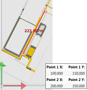
Transforming a Representation Based on the X, Y Coordinates of Two Known Locations

You resize, scale and rotate the map representation using the Reference Points tool:

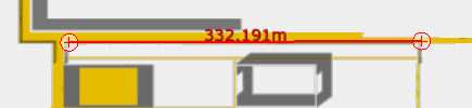
To transform a map representation based on known coordinates:

1. On the Import representations tab, select the map representation.
2. In the workspace, click the TOP VIEW option.
3. Click to turn on Show reference points.
4. Position the two ends of the reference line on the two locations.
5. Enter the X, Y coordinates of the first location in the Point 1 X, Point 1 Y fields.
6. Enter the X, Y coordinates of the second location in the Point 2 X, Point 2 Y fields.

The representation is then transformed. The transformation sets the correct values for:

• size, as shown in the Size X, Y fields
• offset from the origin, as shown in the Origin X, Y fields
• scale factor, as shown in the Scaling X, Y fields
• rotation, as shown in the Yaw field

Defining the Origin

Before you place images, ensure that you define the origin for:

• Background representations: The origin marks the 0,0,0 coordinates that identifies the point, relative to which the sensor positions were measured. Transforming a Map Representation by Using Reference Points describes how to resize, scale, rotate and set the origin of the background representation in one step.
• Other images: You can use the origin to mark the central point of an object, which can make it easier for you to place objects by using absolute coordinates.

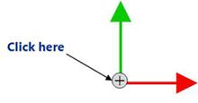
To mark the origin of an image:

1. On the Import representations tab, select the required image.

2. Click and drag the origin to the required position in the image, as shown in the following figure:

   

   The updated X,Y,Z coordinates are displayed on the left.

3. Adjust the origin using the Origin X, Origin Y and Origin Z fields.

Placing Background Representations and Objects

After you have imported and adjusted the required images, you can place these objects as required in the Add background objects tab.

Ubisense-supplied representations for Ident points and GPS reference points are also listed on the left-hand side of the Add background objects tab. For information on using these reference objects, see Adding and Positioning Ident Points and Adding and Positioning Ident Points.

To place objects:

1. Click the Add background objects tab. All the background representations and images that you have imported are listed at the top.

2. Select and drag the background representation to the screen. The background object is listed at the bottom—double-click the object to display an editor in which you can adjust the location and orientation of the background representation.

3. Select and drag additional objects to the screen.

4. Following the onscreen instructions, place and position the additional objects on the background representation, as required.

Deleting an Object

To delete an object, and its representation:

1. Click the Add background objects tab. The Background Object section lists all the representations that you have added and placed.

2. Select the object that you want to delete, and then press the Delete key.

   The object is removed. However, the representation is still retained in the D4 RTLS.

3. To delete the representation:

   1. On the Import representations tab, locate and select the image that you want to delete.

   2. Press the Delete key.

   The representation is removed from your D4 RTLS.

Adding and Placing Devices

You can add DIMENSION4 sensors, Timing Distribution Units (TDUs) and 2.4GHz Receivers to your D4 RTLS.

Adding and placing devices involves:

• Adding each device by specifying its MAC address.

• Creating one or more sensor groups to group the devices logically, and adding each device to the appropriate group.

  Device	Details
  Sensors	Create the required groups, and enter the location of each sensor. You do not need to enter the orientation of the sensors—the Solver will calculate this for you.
  TDU	Automatically added to its own group. Enter the location.
  2.4GHz Receiver	Automatically added to its own group. Enter the location.

• Adding sensors to the appropriate groups.
• Positioning sensors.

Adding and Deleting Devices

You can add a sensor or TDU to the D4 RTLS by either:

• Typing its MAC address.

• Scanning its MAC address from the barcode label.

You can add a 2.4GHz Receiver by typing in its MAC address.

Adding a Device using its MAC Address

To add a device by using its MAC address:

1. On the Place devices tab, add the required device. To add multiple devices, type the MAC address of each device on a separate line.

   LSC automatically detects the type of device and places it in the correct group.

2. Save the MAC addresses that you have typed.

   The device(s) appear on the following lists:

   • Ungrouped: The sensors currently do not belong to any group.

   • Unpositioned: The devices, whether sensors, TDUs or 2.4GHz Receivers do not have a location.

Adding a Device by Scanning its Barcode Label

To add a device by scanning its MAC address from the barcode label on its back panel, you require a 1D Barcode Scanner.

To add a device by scanning its barcode label:

1. Connect the Barcode Scanner to your computer.

2. On the Place devices tab, double-click <Add new device>.

   Make sure that the cursor is displayed in the box.

3. Using the Barcode Scanner, scan the MAC address barcode label of the device.

4. The MAC address appears on the list of devices to be added.

5. Save the address that you have scanned.

   The device(s) appear on the following lists:

   • Ungrouped: The sensors currently do not belong to any group.

   • Unpositioned: The devices, whether sensors, TDUs or 2.4GHz Receivers do not have a location.

Naming Devices

The devices listed on the Place devices tab are listed by name if the name is configured, otherwise they are listed by MAC address.

To enter the name of each device, double-click the MAC address to display the editor.

Deleting a Device

You can only delete a device that is ungrouped.

To delete a device:

1. On the Place devices tab, select the device that you want to delete from the Ungrouped list, and then press the Delete key. The LSC tool prompts you to confirm that you want to delete the sensor.

2. Click Delete.

   The device is deleted. It no longer generates location data or distributes timing.

Working with Sensor Groups

In a D4 RTLS, the entire location tracking area is covered by one or more Sensor Groups. Sensors that belong to the same group can exchange data to locate a tag. Sensors from different groups cannot exchange data.

The size and number of groups that you must create depends on the requirements defined in your sensor installation plan.

Typically, groups are created depending on:

• The size of the location tracking area. A small area might require one group with a small number of sensors, whereas a larger area might require multiple groups and more sensors.

• The way in which you want to track your objects. For example, if objects are moving along a line, you can create overlapping groups, so that the sensors can track objects as they move from one area to another.

About Sensor Groups

A Sensor Group can cover multiple rooms. Sensors can belong to one or more groups.

An example Location Cell with three sensor groups, is shown in the following figure.

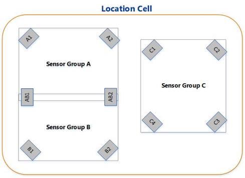
Sensor Groups

In the example:

• Group A and Group B are adjacent to each other (and overlap). Sensors AB1 and AB2 belong to both Group A and Group B. Therefore, these two sensors can exchange data with the other sensors from both Group A and Group B.

• Sensors A1, A2, B1, and B2 are not shared. Therefore, they cannot exchange any data between Groups A and B.

• Group C is completely independent and does not share any sensors or exchange data with Group A and Group B.

A sensor group can overlap location cells but the results can be confusing when reviewing events, because sensors send data to the location cell they are in and the choice of sensor for a tag does not depend on the location of the tag—so event data fro a tag in cell A may go to cell B.

About Clipping Regions and Snap Distances

You can define a clipping region for a Sensor Group if you are only interested in the location events that are generated when tags are inside the area covered by the clipping region.

If required, you can also define a zone around the clipping region, called the snap distance. If a tag is detected inside the snap distance, it is considered to be inside a Sensor Group. Therefore, if a tag enters this zone, sensors can locate the tag even if it is not fully within the group.

As a sensor group represents a 3-dimensional space, you can configure both horizontal snap distance and vertical snap distance for your sensor group. The following figure shows an example for horizontal snap distance.

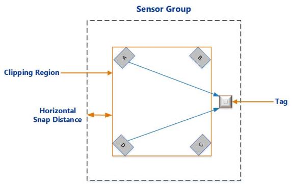
Horizontal Snap Distance

Creating Sensor Groups

To create a sensor group:

1. Click the Place devices tab.

2. Create a new sensor group. To create multiple sensor groups at the same time, type the name of each sensor group, one on each line of the box.

3. Click Save.

   The new groups appear in the list of existing groups.

Defining a Clipping Region

You can optionally define a 2.5D clipping region for each group.

1. Double-click the group.

2. Following the onscreen instructions, add points to define the 2D extent of the clipping region.

   When you click and drag to add a point, the coordinates of the point are displayed. Use this information to place the clipping region within the Location Cell, allowing also for the snap distance that is in addition to the extent.

   Notes:

   • The clipping region can be any shape.
   • If you want to share a sensor between groups that have a clipping region, then the clipping regions should overlap.
   • If you have set up a background representation, you can use this as a guide when defining the 2D extent of the clipping regions.
   • To view coordinates and additional features such as background representations, click Show view options.

3. Specify the height (top and bottom) of the clipping region in meters—this must be contained within the height of the Location Cell.

   The floor of the clipping region must match the actual height of the floor in your physical environment. This floor height is used as a reference to specify the height range for tag filters, as described in Configuring Height and Speed.

4. Optionally, specify the horizontal and vertical snap distances.

Adding a Sensor to a Group

Each sensor must belong to at least one group. You can also add a sensor to multiple groups if you need to track the movement of a tag from an area covered by one Sensor Group into an area covered by another group.

To add a sensor to a group:

1. Click the Place devices tab.

2. Do one of the following:

   • If the sensor does not belong to any group, it appears on the list of Ungrouped sensors. Select the sensor and then drag it into the required group.

   • If the sensor already belongs to a group and you want to share it with another group, press the Shift key, and drag and drop the sensor from one group to another group. The sensor is listed in both groups.

Positioning Sensors

Positioning a sensor in a group involves:

1. Specifying the precise X, Y, and Z coordinates of the sensor.

2. Specifying the approximate pitch and yaw angles of the sensor.

This information is used to calculate tag positions.

Estimating Pitch and Yaw

When placing a sensor, you should specify the approximate pitch and yaw of the sensor. These values are then accurately measured and overridden when you run the Solver, as described in Solving Sensor Parameters.

Pitch

Pitch is the vertical angle of the sensor. Examples of a sensor positioned at a pitch of ‑41 degrees and ‑55 degrees, are shown in the following figure.

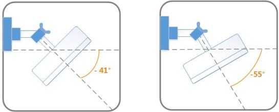
Sensor Positioned at Different Pitch Angles

Yaw

Yaw is the horizontal angle of the sensor, shown in the following figure.

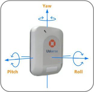
Yaw, Pitch, and Roll of a Sensor

Obtaining Sensor Positions

To calculate the position of a tag, you require the precise X, Y, Z coordinates of each sensor that belongs to the group.

These coordinates are measured with a Total Station and recorded after the sensors are installed.

To calculate the X, Y, Z coordinates of a sensor:

1. Define a coordinate system.
   1. In your location tracking site, pick a point on the floor (origin) from which you can measure the coordinates.
   2. Decide which horizontal direction you want to use as the positive X-axis. Facing in this direction, the positive Y-axis is to your left, and the positive Z-axis is upwards.

2. Following the instructions supplied with your Total Station, measure the position of the fiducial mark on the front panel of the sensor.

   Ensure that you:

   • Measure both horizontal and vertical offsets to the sensor.
   • Survey the positions of the sensor to an accuracy of better than 5 cms. If the surveyed positions are accurate, the Solver (part of Location System Config) returns more reliable sensor positions.
3. Note down the coordinates for the X, Y, and Z axes, for example, add them to the Sensor Installation Plan.

Positioning the Sensor

Sensors that do not have a location appear on the list of Unpositioned sensors (even if they already belong to one or more groups).

To position a sensor:

1. On the Place devices tab, double-click the MAC address or name of the sensor.

2. Define its position by specifying the location, yaw, and pitch.

   Field	Value
   Location	Type the X, Y, and Z coordinates with the values that have been calculated with a Total Station. Note that: The coordinates must be inside a Location Cell. You can drag the sensor from the Unpositioned list onto the map.
   Yaw and Pitch	Type the estimated horizontal and vertical angles at which the sensor has been mounted or enter 0. For more information, see Estimating Pitch and Yaw.

Removing a Sensor from a Group

To remove a sensor from a group:

1. Expand the group from which you want to remove the sensor.

2. Select the sensor, and then press the Delete key.

3. The sensor is removed from the group.

   Note that the sensor appears on the list of Ungrouped sensors only if it does not belong to any other group.

Unpositioning Sensors

To unposition a sensor:

1. On the Place devices tab, double-click the MAC address or name of the sensor that you want to unposition.

2. Select the Unset sensor position check box.

3. Save the settings.

   The sensor still belongs to the group but it no longer has any coordinates, and therefore appears on the list of Unpositioned sensors.

4. You can now reposition the sensor as required.

Deleting a Sensor Group

To delete a Sensor Group:

1. On the Place devices tab, select the group that you want to delete, and then press the Delete key. The LSC tool prompts you to confirm that you want to delete the group.

2. Click Delete.

The Sensor Group is deleted. If the sensors do not belong to any other group, they appear on the list of Ungrouped sensors.

Positioning Other Devices

TDUs

You must set the position of TDUs as this ensures that they are displayed in the correct location on the background map.

A TDU does not need to be positioned in the same Location Cell as its sensors. You do not have to specify the orientation of a TDU as TDUs do not locate tags.

To position a TDU:

1. On the Place devices tab, expand the TDU group.

2. Do one of the following:

   • Double-click the TDU that you want to position, and then type its X, Y, Z co-ordinates.
   • Drag the TDU to the map.

   Ensure that you position the TDU within the extent of a Location Cell.

2.4GHz Receivers

For information on positioning receivers, see Configuring 2.4GHz Receivers.

Configuring Timing

Sensors use timing signals to record the precise time at which they detect a UWB pulse from a tag and then generate TDOAs that are used for identifying the tag location.

Configuring timing involves:

1. Setting up one or more sensors as timing sources.

2. Defining how other sensors receive timing signals.

Timing Sources and Timing Trees

The timing signal is always generated by a sensor that has been designated as a timing source. The timing source is at the root of a timing cable tree, and provides synchronization signals to all the downstream or recipient sensors in that tree.

When two sensors are connected with a timing cable, the upstream (supplying) sensor controls the timing signal and transmits its MAC address to the downstream (receiving) sensor. The sensors therefore detect the topology of the timing tree automatically.

Ideally all the sensors in a Sensor Group belong to the same timing tree.

If necessary, a group can have multiple timing sources and timing trees, as shown in the following figure.

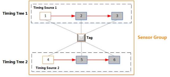
Multiple Timing Trees in the Same Group

The figure shows an example sensor group that has six sensors and two separate timing trees:

• Sensors 2 and 3 receive timing signals from Timing Source 1. They are synchronized with each other and generate TDOAs.

• Sensors 5 and 6 receive timing signals from Timing Source 2. They are synchronized with each other and generate TDOAs.

Configuring Timing Sources

The sensor installation plan defines the timing sources and cabling for each group. Each group can have multiple timing sources and timing trees.

To set up a sensor as a timing source:

1. On the Configure timing tab, identify the sensor that must be configured as the timing source.

   By default, all sensors are configured to receive timing signals through a cable.

2. Select the sensor that must be configured as a timing source. From the Timing drop-down menu, select Timing source.

3. Reboot the sensor, as described in Rebooting Devices.

   You must reboot the sensor whenever you change the timing source.

The timing status of the sensor is updated. The sensor now only generates timing signals, which can be used by other sensors.

Configuring Timing Options for Sensors

Sensors can receive timing either through an Ethernet cable or a timing cable.

Receiving Timing through a Timing Cable

By default, a sensor is configured to receive timing through a timing cable.

On the Configure timing tab, choose the Receive from cable option from the drop-down list if either:

• The sensor has been daisy-chained, where it receives timing signals from another sensor that is connected to the timing source.

• The sensor receives timing signals directly from the timing source.

For information on configuring sensors and cables, see Connecting Network and Timing Cables to Sensors.

Receiving Timing from a TDU

If you are using a TDU to distribute combined network and timing signals, you must change the timing configuration for the sensors.

To do this, on the Configure timing tab, change the timing status to Receive from ethernet.

Configuring Timing Sources for Use with TDUs

You can use a sensor to distribute combined network and timing signals through the Ethernet cable (connected to the Ethernet (PoE) port on the sensor) as shown in the following figure.

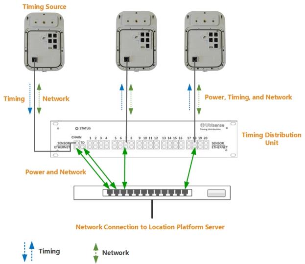
Hardware Configuration for Distributing Timing on the Ethernet Port

For this setup, change the timing configuration as follows:

1. On the Change sensor parameters tab, select the sensor to use as the timing source.

2. Navigate to the Sensor > Physical > Timing > Allow Ethernet Output parameter.

   The parameter has the following values:

   • False: the sensor is configured for timing input only on the Ethernet port.
   • True: the sensor is configured to send timing output on the Ethernet port, if it does not receive timing from this port.

3. Double-click Allow Ethernet Output and set the parameter as required:

   • To configure the sensor for both timing input and output, select the check box.
   • To configure the sensor for timing input only, clear the check box.
4. Click Save.

Checking and Troubleshooting Timing Trees

After you have set up timing sources and defined timing options for the other sensors in the group, check the timing trees to see how the timing signals are distributed.

On the Place devices tab, click Show view options, and then select Show timing tree.

Red arrows, which indicate timing signals, are shown on the sensor group:

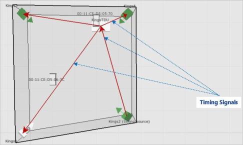
Sensor Group Showing the Timing Tree

The directions of the arrows show how the timing signals are distributed. Review the timing tree carefully to check that the timing signals are distributed, as expected.

If the arrows fail to appear or do not appear as you expected, check for any obvious issues, for example:

• Check that you have set up correct timing sources and cabling options for sensors.

• Check that the physical cables have been connected to the correct ports on the sensors, as described in the DIMENSION4 website at https://www.ubisenseDIMENSION4.com.

Sensor Network Configuration

All devices in your D4 RTLS are connected by means of network cables and require a network connection to exchange data. They must also be able to connect to a Location Platform server in order to obtain configuration information for booting.

By default, each device receives its IP address, subnet mask, and default gateway from a DHCP server. Alternatively, you can configure a device to connect to the Location Platform server by assigning:

• A static IP address, subnet mask, and default gateway.

• A DNS configuration, which can contain up to four DNS server IP addresses and up to four suffixes to use.

• A particular search order, which contains a sequence of different methods, such as a simple domain name, fully qualified domain name, IP address, or broadcast, which the device can use to contact the Location Platform server.

Creating a Search Order

The search methods that you can use are listed in the following table.

Search Method	Device connects to the network by...
Simple domain name	Using a domain name that resolves to an IP address known to the DNS server.
Fully-qualified domain name	Using a domain name that specifies its exact location in the tree hierarchy of the Domain Name System (DNS).
IP Address	Using the IP address of the Location Platform server.
Broadcast	Searching for any available Location Platform server on the same sub network.

To set up a search order:

1. On the Sensor network configuration tab, add a new search order, ensuring that you provide a unique name for the search order.

2. Add the required search methods in the order that they should be used.

3. Review the details that you have typed.

   It is not possible to modify a search order after you save it. To modify an existing search order, you must delete it and then create a new search order with the required settings.

4. Save the search order. The new search order appears on the list of Search Orders. You can add the search order to the required devices.

Creating a DNS Configuration

To create a new DNS configuration:

1. On the Sensor network configuration tab, create a new DNS configuration.

   For example, name it ubisenseconfig.

2. Add up to four DNS IP addresses or DNS Suffixes or both, as required.

3. Review the details you have typed.

   It is not possible to modify a DNS configuration after you save it. To modify an existing DNS configuration, delete it and then create a new configuration.

4. Save the DNS configuration.

5. Assign the DNS configuration to the required devices. See Assigning Network Settings to Devices.

Assigning Network Settings to Devices

All devices that currently do not have any custom network configuration are listed in the Default group. These devices use DHCP settings by default.

To assign custom network settings to a sensor or TDU:

1. On the Sensor network configuration tab, select the required device.

2. The device can support a valid combination of settings, as listed in the following table.

   IP Address	Subnet Mask	Default Gateway	DNS Config	Search Order
   -	-	-	-
   		-	-	-
   		-	-
   		-		-
   		-
   			-	-
   			-

3. Save your settings.

   The device is listed under the pending validation group until the static IP settings and/or DNS configuration are validated. If the settings are valid, the device is listed under the valid group.

Notes

If you left any fields blank, the device connects to the server as described in the following table.

If you did not specify...	Behavior
IP address and subnet mask	The device connects to the Location Platform server by using DHCP.
Default gateway	If you have not specified an IP address and subnet mask, the device obtains the gateway IP address by means of DHCP. If you have specified an IP address and subnet mask, the device will not have a gateway IP address. The device can only contact the Location Platform server in its subnet.
DNS configuration	If you have not specified an IP address and subnet mask, the device obtains the DNS configuration from a DNS server. If you have specified an IP address and subnet mask, the device will not perform any DNS queries.
Search order	The device uses the default Ubisense search order.

Network Statuses

After you have assigned network settings to a sensor or TDU, it appears under one of the network status groups that are listed in the following table.

Network Status Group	Description
Custom (valid)	The device has successfully validated the network settings.
Custom (pending validation)	The network settings are awaiting validation from the device.
Custom (invalid)	The device could not validate the network settings.
Default	The device is using the default network configuration (DHCP). Custom network settings have not been specified.

Deleting DNS Configurations and Search Orders

You can only delete DNS configurations and search orders that are currently not used by any device.

To delete an existing DNS configuration or search order:

1. Identify the devices that are currently using the specific DNS configuration or search order. Remove the DNS configuration or search order from the network settings of each device.

2. From the list of DNS Configurations, select the configuration that you want to delete, and then press the Delete key.

   The DNS configuration is removed from the list.

Setting up DHCP Servers

Sensors and other Ubisense hardware, such as Timing Distribution Units and 2.4GHz Receivers, require a network infrastructure to communicate with the DIMENSION4 Real-time Location System (D4 RTLS).

Although not essential, the default configuration for the D4 RTLS uses DHCP and DNS servers to:

• Dynamically assign IP addresses to sensors.

• Enable sensors to determine the IP address of the Location Platform server.

The D4 RTLS does not rely upon either DHCP or DNS being available. In these situations, you can assign static IP addresses to each sensor.

Once the sensors and TDUs have been installed and connected, the network settings are configured using the Ubisense Location System Config tool (LSC).

DHCP Server

A DHCP server is used for assigning IP addresses to the sensors, TDUs and 2.4GHz Receivers.

As a minimum, the DHCP server must provide the following information to a sensor:

• IP address

• Subnet mask

• Gateway IP address

Solving Sensor Parameters

After you have booted the sensors successfully, you can calculate the orientation and timing for the sensors by running the Solver. During this process, the Solver calculates:

• The yaw and pitch for each sensor, to determine the correct angle at which the sensors receive signals from a tag.

• The cable delay or the time required for the timing signal to reach each sensor. This delay must be calculated to determine the TDOA.

The D4 RTLS uses these values to identify the location of tags.

To run the Solver:

1. Place a tag in a known position.

2. Run the Solver to calculate the yaw, pitch, and cable delay values for the sensors that can see the tag and which are in the same timing tree.

You can run the Solver multiple times for the same sensors. Each solver run captures statistics from hundreds of readings. The D4 RTLS uses the best results based on the lowest standard deviation.

The Solver results of individual sensors affect the group summary. Therefore, you must also run the Solver after you have:

• Physically moved a sensor and recorded the move on the Replace infrastructure tab.

• Replaced a timing cable and recorded the swap on the Replace infrastructure tab.

Running the Solver for the Correct Sensors

The Solver calculates the sensor orientation and cable delay values based on the specific position of a reference tag.

When you run the Solver, it lists all the sensors that can detect signals from a reference tag. If one or more sensors only have a partial line of sight to the tag (see the following example), the Solver might return inaccurate results for those sensors. Therefore, ensure that you run the Solver only for those sensors that can directly sight the tag.

An example sensor group that contains sensors with different orientations, is shown below.

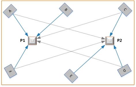
Choosing Sensors when Running Solver

In this example, the sensor parameters are solved with the tag at two different positions, P1 and P2. The sensors can sight the tag as summarized in the following table.

Tag Position	Direct Line of Sight	Partial Line of Sight
P1	Sensor A, Sensor B, and Sensor F	Sensor C and Sensor D
P2	Sensor C, Sensor D, and Sensor E	Sensor A and Sensor F

If you solve parameters with the tag at P1, the Solver lists Sensors C and D, even though they can only sight the tags partially. If you include these sensors in the Solver run, the orientation results for these two sensors will be inaccurate.

To obtain accurate results for Sensors C and D:

• Exclude these sensors from the Solver run when the tag is at P1.

• Solve parameters for these sensors when the tag is at P2.

Prerequisites

Before running the Solver, ensure that you have:

• Configured logging, as described in Configuring Logging. This enables the Solver to obtain data from sensors.
• Added sensors to groups and positioned them, as described in Positioning Sensors. This enables the Solver to calculate orientations and cable delays.
• Configured timing and set the appropriate sensors as timing sources, as described in Configuring Timing Sources.

Running the Solver

Before you begin:

• Place a tag in a position at which the sensors can sight it.

• Ensure that you have the tag ID and the position of the tag in meters.

To calculate accurate orientation and timing values for each sensor that can see the tag:

1. Run the Solver.
2. Review, accept, and save the required results.
3. Check that the tag is being accurately located, and then close the solver run.

Start a Solver Run

To start a Solver run:

1. On the Solve sensor parameters tab, click Solve.

   Notes:

   • If you have not yet run the Solver or if a sensor from a group does not have any result (for example, it cannot detect the tag), then the group summary appears as Incomplete.

   • To view the Solver status of individual sensors from the group, expand the group. Sensors that do not have any results show:

     • The estimated pitch and yaw, if you have provided these values.

     • A timing result of Not done.

2. Type the complete tag ID and the X, Y, Z coordinates (in meters) of the tag that you have placed, and then click Start.

   Notes:

   • It can take some time for all sensors to appear on the screen.

   • Results are only displayed when you select the check boxes for one or more of the sensors listed in the Store results area.

   • The Solver captures statistics from hundreds of readings for the selected sensors. The values displayed on the screen are continuously updated based on new readings. The values stabilize when the readings are consistent.

3. The next step is to review and accept the results.

Review and Accept Results

After running the Solver, the Solve sensor parameters tab shows results for the selected sensors, in a three-column layout, as shown in the following example:

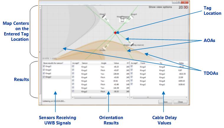
Solver Window

 

To review and accept results:

1. In the first column, the Solver lists all the sensors that can detect UWB signals from the tag. Select only those sensors that have a direct line of sight to the tag (see Running the Solver for the Correct Sensors).

2. In the second column, the Solver lists the calculated pitch and yaw for each sensor. Select the results that you want to use.

   Notes:

   • Even if the standard deviation is low, accept the results only if they correspond to the physical orientation of the sensors.

   • If the results of a sensor are consistently poor:

     • Solve parameters for the sensor by placing a tag in a different measured position.
     • Check and adjust the physical orientation of the sensor, if necessary.
     • Check if there are any obstructions that might affect the ability of the sensor to sight the tag.

3. In the third column, the Solver lists the cable delay between sensor pairs—select all the check boxes in this column.

   Notes:

   • The results for a sensor pair do not appear if a timing signal path from the sensors to the timing source does not exist.

   • If the results are not generated or are consistently poor:

     • Check that you have set up correct timing sources and cabling options for sensors.
     • Check that the physical cables have been connected to the correct ports on the sensors, as described in Connecting Network and Timing Cables to Sensors.

4. When the readings are stable, save the results.

   The results displayed on the screen are updated even after you save your solver run. If you click Save again, the new results replace the existing values in your solver run.

5. The next step is to check the results of the operation.

Check the Operation

After saving the solver run, check its outcome.

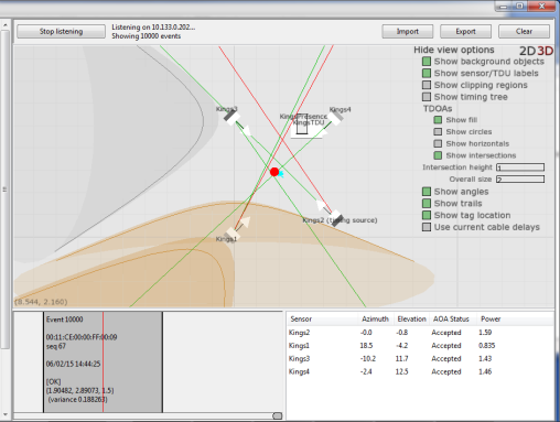
The following screenshot shows an example of sensors with OK results.

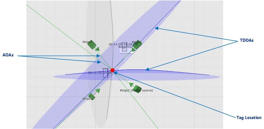
Sensors with OK Orientation Results

Orientation Results

The color of the sensor shows the orientation results for that sensor:

• Green: the orientation results are acceptable (OK).
• Yellow: the orientation results are poor.
• Grey: there are no orientation results.

The TDOAs and AOAs show that the filter is using the results when:

• The color of the TDOAs changes to blue. The TDOAs also intersect at the tag location.

• The color of the AOAs is green.

For information on setting up filters, see Setting up Tag Filters.

Timing Results

To check the timing results, close the solver run, and review the information shown in the summary table.

Reviewing Solver Status

The Solver records the sensor orientation and timing (cable delay values) for the group as a whole and also individual sensors from the group. The result of an individual sensor affects the overall result of its group. For example, if a sensor does not have a result, the summary of the entire group appears as Incomplete.

Sensor Results

The possible Solver results for sensors are summarized in the following table.

Sensor Summary	Description
OK	The results are acceptable, as they have a low standard deviation.
OK (Partition N)	This indicates that timing has been solved for separate sets of sensors within a group (i.e. the partitions) but that there is not enough information to calculate timing between these sets. This will lead to inability to compute TDOA for sightings involving sensors from the different sets. Resolving this requires running the solver for a tag located in sight of some sensors from both sets.
Not done	The sensor does not have any Solver results yet.
Poor	The results have a high standard deviation and therefore may or may not acceptable. For information on resolving poor results, see Review and Accept Results.

Sensor Group Summary

The possible statuses for sensor groups are summarized in the following table.

Group summary	Description
OK	All sensors from the group have acceptable results.
Incomplete	A sensor group has this status when: One or more sensors from the group do not have a result. Timing has been solved for separate sets of sensors within a group, but with insufficient information to calculate timing between these sets. All the results have been rejected.
Poor	The results for one or more sensors from the group are poor. For information on resolving poor results, see Review and Accept Results.

Viewing and Modifying Solver Runs

You can modify existing Solver runs to accept or reject individual values that were calculated for a particular sensor.

To view and modify a solver run:

1. On the Solve sensor parameters tab, select the required sensor group or sensor. All solver runs that apply to the selected sensor group or sensor are listed.

2. To view or modify a solver run, double-click the required solver run.

   The solver run lists the yaw, pitch, and cable delay values for all sensors that were included in that run.

3. Accept or reject the values as required.

   To reject a result, clear the Accept? check box.

4. Close the solver run.

   The status of the sensor and its group are updated.

Notes

• The overall pitch, yaw, and cable delay values of a sensor are calculated from multiple solver runs. When you modify a solver run, the overall values are recalculated.

• If sufficient readings or solver runs are not available for determining the pitch, yaw, and cable delay values of a sensor:

  • The sensor shows the estimated yaw and pitch and/or a timing result of Not done.

  • The orientation and/or timing status of the sensor group changes to Incomplete.

Setting up Tag Filters

A filter is a set of rules and conditions that you can configure to define, for example, the height at which the tag is likely to be found, and the speed at which the tag is likely to move. These filters are used by sensors to sight and track tags.

To configure and apply a tag filter:

1. Create a filter.

2. Configure the required parameters, including the height, speed, and model type for the filter.

3. Optionally, experiment with different values to obtain better locations, by using command-line tools—see the advanced documentation described below.

4. Apply the filter to either a tag, a tag type, or a range of tags.

Creating a Filter

You can set up a filter for either a particular tag, a tag type, or a range of tags. To configure different filter settings for different sets of tags, ensure that you create a separate filter for each set of tags.

To create a filter, on the Set up tag filters tab, add a new filter and then configure filter parameters to define how the tags must be tracked.

Configuring Height and Speed

For each filter that you create, configure the height and speed parameters that are listed in the following table.

Parameter	Description
Default Height	This height is used during initialization, if the true height of the tag cannot be determined. If you are not sure which value to use, specify a value that lies half way between the maximum height and minimum height.
Horizontal Speed	The maximum speed at which the tag can move, before the calculated position starts to lag. We recommend that you set this value to slightly higher than the fastest speed at which the tag is likely to move. If you set this to a very high value, the reported location jumps too quickly in response to new measurements.
Maximum Height	The maximum height that the tag is likely to reach. Any sightings of a tag that are above this value will be rejected.
Minimum Height	The minimum height that the tag is likely to reach. Any sightings of a tag that are below this value will be rejected.

Height

• Although the maximum and minimum heights do not have to be very accurate, ensure that they are approximately the same as the actual heights at which the tags are used. For example, for tool tags that are carried by people:

  • 0.5 m (knee height).

  • 1.0 m (waist height).

  • 1.5 m (shoulder height).

• If the sensor groups have a clipping region, ensure that the height that you specify is in relation to the floor of the clipping region of the sensor group that detects the tag. If you have set the height of sensors and the clipping regions to the correct absolute heights, the same filter parameters will work, for example, if the tag is used on two different floors of the same building.

Speed

Use an estimated value for the speed at which the tag is likely to move. A common value that you can use for speed is 2.5 m/s (5.5 mph or 9 kph), which is slow jogging speed.

Setting the Motion Model

The Model Type parameter specifies the motion model, which is used for extrapolating the movement of the tag.

Option	Description
1 (Planar)	The tag position moves in a fixed-height horizontal plane.
2 (Stationary)	The tag can move horizontally and vertically, with a minimum and maximum height limitation. Always select this option for all regular location tracking scenarios.

Applying a Filter

You can apply a filter to either:

• A tag range, by specifying the filter to be assigned to a range of tag IDs.
• A tag type, by specifying the filter to be assigned to a tag type (this takes precedence over a tag range).
• A particular tag, by specifying the filter to be assigned to a specific tag ID (this takes precedence over a tag type).

Tag ranges must not overlap. However a tag range that is a subset of another tag range is supported, as shown in the following example.

Filter Range	Supported (Yes/ No)
Filter 1 range: 00:11:CE:00:00:00:01:00 to 00:11:CE:00:00:00:01:FF Filter 2 range: 00:11:CE:00:00:00:01:C0 to 00:11:CE:00:00:00:02:40	No. The tag ranges overlap from 01:C0 to 01:FF.
Filter 1 range: 00:11:CE:00:00:00:01:00 to 00:11:CE:00:00:00:01:FF Filter 2 range: 00:11:CE:00:00:00:01:C0 to 00:11:CE:00:00:00:01:DD	Yes. Tags in the smaller range use Filter 2. Tags in the larger range (excluding tags in the smaller range) use Filter 1.

To apply a filter to a tag, tag type or tag range:

1. On the Set up tag filters tab, do one of the following:

   • To apply a filter to a set of tags, double-click <Add new tag range>. Specify the range of tag IDs, in hexadecimal format.

   • To apply a filter to a tag type, double-click <Add new tag type>. Specify the name of the tag type, and (optionally) the name of a different tag type to use as a template for this new tag type.

   • To apply a filter to a particular tag, double-click <Add new tag>. Specify the tag ID, in hexadecimal format.

     You can find the tag ID on its case.

2. Apply the required filter.

3. Save your changes.

The sensors start tracking the tag, the set of tags, or tag types according to the filter settings.

Checking Filters

To check that the filters are working as expected:

1. Review events, as described in Reviewing Location Events.

2. Check the performance of filters by comparing new events with previous events.

   You can also use command-line tools for this.

Viewing the Device Status

Sensors and TDUs that are connected to the network, and receiving power through Power-over-Ethernet (PoE), will have Running status if you have:

• Created the required Geometry Cells and Location Cells.

• Positioned the devices within Location Cells.

• Configured network and timing for the devices.

The actual status of the sensors in the different Location Cells will differ depending on the completeness of the configuration.

To view the status of a sensor or TDU, click the View sensor status tab.

Device Statuses

A device that has Running status has booted successfully.

The following statuses indicate that you have configured the device but there is a specific problem that you need to resolve:

Status	Description
Last seen booting	The device was rebooted at the specified date and time. This means one of the following: The device is either in the process of booting. The device has failed to boot successfully. See Troubleshooting Booting Errors.
No timing signal	The device has booted successfully, but is not receiving a timing signal.

These statuses indicate a more fundamental problem:

Status	Description
Last seen...	With the exception of Last seen booting, there is problem preventing the system from reporting the current status. For example, there may be no network connection.
No geometry cell No location cell	The device is not located in a geometry cell or location cell so it cannot obtain its configuration settings from the server. It will continue to reboot until it has obtained its configuration.
Unknown	The device may not be connected to the network.

Notes on the View sensor status tab:

• The Status Age indicates the duration for which the device has been in its current status.

• You can sort sensors by clicking the column headings.

• You can group sensors by using the Group by option.

• You can optionally add comments to individual devices or sets of devices.

Adding Comments to Devices

You can add a comment to one or more devices listed on the View sensor status tab.

To add a comment to a single device—double-click the device to open the editor.

To add a comment to several devices:

1. Press the Shift or Ctrl keys and then click the required devices.
2. Click Edit comment.

Troubleshooting Booting Errors

Sensors and TDUs have the same operating and statuses and error codes. These are described in DIMENSION 4 boot process overview

LED Error Codes and Timing Trees

In a timing tree, the upstream sensor distributes timing to the downstream sensors. If the upstream sensor is not working, the downstream sensors do not receive timing and the LEDs will flash green/orange (notice that this is not an LED error code). Therefore, when troubleshooting any booting errors, first examine the timing tree for any potential problems.

Rebooting Devices

To reboot sensors and TDUs:

1. On the View sensor status tab, select the device that you want to reboot. To reboot multiple devices: press the Shift or Ctrl keys and then click the required devices.

2. Click Reboot.

The status of the device first changes to Rebooting then, after the device is booted successfully, the status changes to Running.

When handling a large number of sensors, it is useful to group the sensors first. For example, to reboot sensors in a sensor group and then observe their status:

1. Group the sensors by Group.

2. Select the sensors in the Group, and then click Show selected.

3. Click Reboot.

4. Group the sensors by Status, and then click Expand all. The progress summary of only those sensors that you have rebooted is then displayed.

5. When you have finished, click Show all.

Reviewing Location Events

You can check the location of tags by reviewing either:

• Historical events, which show the location history of one or more tags.

• Real-time events, which show the current location of one or more tags.

When data is retrieved using filters, the filtering is done on the server side, so that it is possible to pull back complex queries without putting lots of data on the network. In general it is incorrect to try to work out how well a system is performing by looking at the events files. It is a much better approach to use the offline scriptable analysis tools described in Filter Configuration.

Getting Location Events

Listening in Real Time

When you listen in real time, you can review the events as and when they are generated by the sensors.

To view the location of tags in real time:

1. On the Review location events tab, clear the display if required.

2. Click Get events.

   Notice the maximum number of real-time events to display. We recommend that you do not normally change this.

3. Select the Listen in real time option.
4. Select the Location Cell.

5. Click Start listening.

6. Monitor events as they occur. See Reviewing Location Events.
7. When you have finished, click Stop listening.

8. You can now:

   • Save the events by exporting them to an event file. See Exporting Location Events.
   • Filter the events to show just a subset of the events. See Filtering Messages.

Retrieving Historical Location Events

To view historical location events:

1. On the Review location events tab, if necessary click Clear.

2. Click Get events.
3. Enter the maximum number of events to retrieve.

4. Select the Use last or Enter timespan options.

5. Select the Location Cell.

6. Click Retrieve Messages.

   After all the location events within the timespan are retrieved, the button changes back to Get events.

7. Review the events that have been retrieved.

8. You can now:
• Retrieve events for other Location Cells, and LSC will merge them into the time line, in chronological order.
• Load events by importing them from an event file.
• Filter the events to show just a subset of the events.
• Export the events in the time line.

Filtering Messages

To filter location events that you have retrieved whether real-time or historical:

1. Click Get events.
2. In the Times section, select Filter messages that have already been retrieved.

3. In the Filters section, enter a Tag ID.

   You can also set up advanced filter controls if necessary. To do this, click Switch to advanced filter controls and then follow the onscreen instructions.

4. Click Filter Messages.

You can now review the filtered messages.

Troubleshooting

If no event data is displayed, check that the machine on which LSC is running is listening on the correct port or network interface card (NIC)—the correct NIC is the one that connects via the network to the Location Platform server. If the incorrect NIC is being used, the top line on Events page shows that the IP address is 0.0.0.0: <port>.

To obtain the IP address of the NIC that LSC is currently using: on the Review location events tab, start listening in real time. The IP address is shown in the top left of the tab.

If necessary, you can set the correct IP address of the NIC in the Windows registry:

1. In the Windows Registry Editor, go to Computer > HKEY_LOCAL_MACHINE> SOFTWARE > Wow6432Node > Ubisense 2.1 > Platform > Config.
2. Add a new registry entry (String Value) called platform_interface.
3. Set the value of the entry to the IP address (for example, 10.42.55.66) of the NIC connected to the Location Platform server.
4. Restart the Location Platform services.
5. Restart the LSC.

Reviewing Location Events

To review location events, scroll through the time line. You can:

• Use the horizontal scroll bar.
• Press the Left or Right Arrow keys.
• Press the Page Up or Page Down keys.

You can also jump to a specific event by typing in the event number.

OK Orientation and Timing Results

A sensor will generate events by using the measurements shown in the following screen shot.

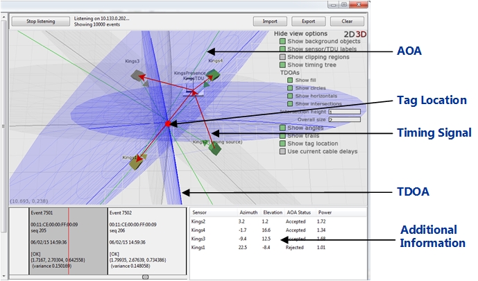
Events Generated by Sensors with OK Solver Results

For these sensors:

• The TDOAs are blue and the TDOAs intersect at the tag location.

• The AOAs are green.

If you have chosen to review events for multiple tags, the red dot on the screen moves from one location to the other, indicating the individual location of each tag.

Poor Orientation and Timing Results

A sensor with results that are poor, or not done, can still sight tags and generate events based on the estimated sensor orientations that you might have provided. However, some of the TDOAs are rejected.

Events of this type are shown in the following screen shot.

Events Generated by Sensors with Poor Solver Results

In this situation:

• The TDOAs are in amber.

• Some of the AOAs are red, which indicate that they are being rejected.

Importing Location Events

You can import location events from saved event files, for diagnostic purposes.

To import location events:

1. On the Review location events tab, click Import.

2. Open the required location events file (.ubievents file).

   Do not increase the number of events to import above the displayed maximum. Your PC may run out of memory if you do so.

3. Click Import.

   The location events from the events file are displayed on the screen.

Exporting Location Events

You can export location events to store the location history of a tag for diagnostic purposes. 

To export location events:

1. On the Review location events tab, click Get events.

2. Retrieve the required location events, as described in Getting Location Events.

3. Click Export, and then save the location events as a .ubievents file.

Setting up Ident Sensors

UWB sensors produce a location event by sharing data with other sensors in a group. In contrast, an Ident sensor produces the location of a tag from a single AOA, without any timing synchronization.

You can use standard Ident sensors if you simply want to determine whether or not a tagged object is inside a certain area, for example, if a car is inside a particular work area such as a Test or Rework Bay. Ident sensors can also be used for tag association and disassociation, where an object is located in an area that is remote from the UWB sensors.

You can use enhanced Ident functionality to detect the presence of tagged objects at one or more defined points in space by using Ident sensors in conjunction with Ident points. For example, with one Ident point you can detect one or more tags at a particular location. Alternatively, by defining an exclusion factor, you can configure an Ident point that only ever contains one tag at a time. (Note that exclusion works on a per-sensor basis. That is sensor A will only put one tag at ident point I, and sensor B will only put one tag at ident point I, but the two sensors may each simultaneously put two different tags at that ident point.)

Using two Ident points with an Ident sensor would enable you to detect a fast-moving tagged object and its direction of travel, for instance when passing through a gate.

You can use an Ident sensor either on its own, or in conjunction with other Ident and/or non-Ident sensors.

How Ident Sensors Generate Location Events

Standard Ident Sensors

A standard Ident sensor generates a valid location when:

1. It receives a signal from the tag and the signal strength is above the configured Power Threshold (see Configuring Ident Parameters).

2. The AOA from the Ident sensor to the tag intersects with the height of the tag, which is determined by the Ident parameter Tag Height (see Configuring Ident Parameters).

The following figure shows an example of a valid location.

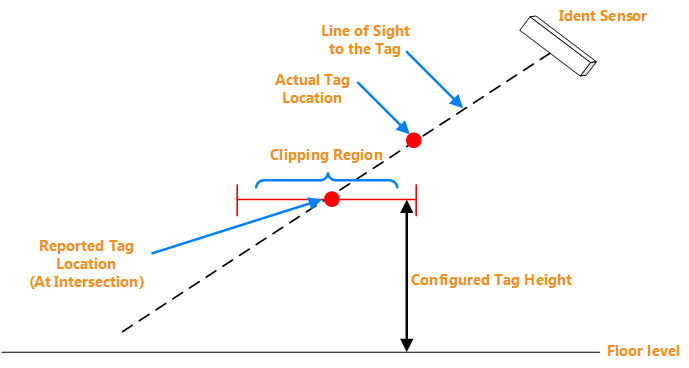
Valid Location Generated by an Ident Sensor

Invalid Locations

If the AOA does not intersect with the clipping region, the location event is reported as Invalid with the message Discarded by clipping region.

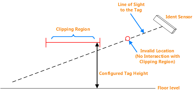
Location is Reported as Invalid

Enhanced Ident Sensors

An enhanced Ident sensor generates a valid location when:

1. An Ident point exists within the 3D clipping region of the Ident sensor's group.
2. It receives a signal from the tag and the signal strength is above the configured Power Threshold (see Configuring Ident Parameters).
3. The tag's location is within the inclusion range for the Ident point.

If a valid location is generated, the tag's location is put at the location of the relevant Ident point.

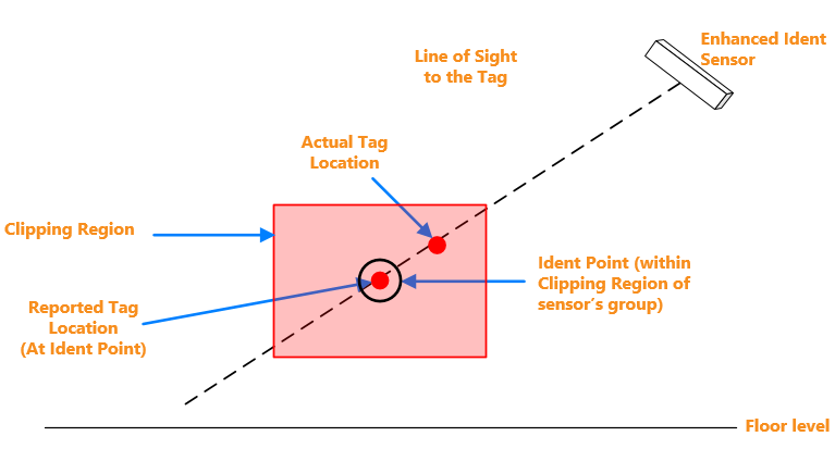
Valid Location Generated by an Enhanced Ident Sensor

Groups

Ident sensors can either work individually or in conjunction with other Ident and/or non-Ident sensors.

Ident Groups

Regardless of whether an Ident sensor works individually or with other sensors, you must first add it to an Ident group.

The following rules apply to Ident sensors and groups:

• An Ident sensor can only belong to one Ident group.

• An Ident group can contain several Ident sensors. Factors such as the size of the tracking area and whether or not sensors have an uninterrupted line of sight to the tag (i.e., the sensors can see the tag clearly without any obstructions) determine the number of sensors in an Ident group.

• An Ident group with standard functionality detects the presence of tagged objects within its 2D clipping region whilst an enhanced Ident group detects tags near Ident points within its 3D clipping region.
• A D4 RTLS can contain several Ident groups.
• Ident groups and non-Ident groups can co-exist in the same D4 RTLS.
• To use Ident sensors in conjunction with non-Ident sensors, you must add the respective Ident groups to a Snoop Group.

Snoop Groups

If an Ident sensor is located close to other non-Ident sensors, both the Ident sensor and non-Ident sensors generate different locations at the same time, causing the tag location to jump. The Snoop group suppresses unwanted location events by acting as arbitrator when there are tag sightings generated by multiple sensors. It ensures that if an Ident sensor receives the strongest signal, then only that sensor generates a location event. Snoop groups can contain both standard Ident groups and enhanced Ident groups.

The following example shows how a Snoop group arbitrates between the tag sightings for tags T1 and T2.

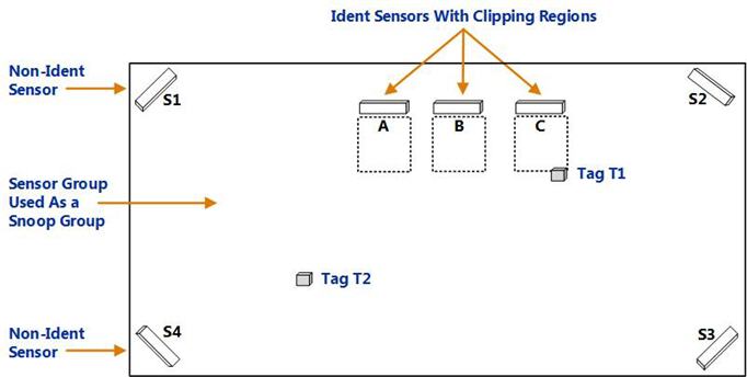
Example of a Snoop Group Arbitrating Between Tag Sightings

In the above example of a Snoop group:

Tag	Sensor	Result
T1	Ident sensor C receives a stronger signal than: Ident sensors A and B Any of the non‑Ident sensors	If there are multiple Ident sensors within the same Ident group, only the sensor that receives the strongest signal will generate a location. Therefore, Ident sensor C can generate a location event for tag T1. The reported location is at the intersection of the AOA with the clipping region of the Ident group.
T2	Non-Ident sensor S4 receives the strongest signal.	The non-Ident sensors in the Sensor group contribute to the location event recorded for tag T2.

Configuration Overview

An Ident sensor is a UWB sensor configured to produce a location of a tag from a single AOA that intersects with a 2D clipping region.

Configuring an Ident sensor involves:

1. Creating an Ident group, if you do not have one already.
2. Adding the sensor to the Ident group.
3. Optionally, creating a Snoop group in scenarios where you want to arbitrate between the readings generated by multiple sensor groups that are located close to each other.
4. Configuring Ident parameters including the Tag Height and Power Threshold.

An enhanced Ident sensor is a UWB sensor configured to produce a location of a tag from a single AOA in proximity with an Ident point that is located in a 3D clipping area. In addition to the steps described above, configuring an enhanced Ident sensor requires the positioning of one or more Ident points within the clipping region of the sensor's Ident group (see Adding and Positioning Ident Points).

The configuration steps are described in detail in the next few sections.

Creating an Ident Group

1. On the Place devices tab, create a new sensor group.

2. Enter the following details, and then click Save.

   Option	Description
   Name	A name for the group. The text (ident group) is displayed next to the name.
   Make these ident group(s)	Select this check box to create the group(s) as Ident groups.

   The Ident group appears on the list of existing groups.

3. Double-click the Ident group to edit its properties.

   1. Draw the boundaries of the clipping region to constrain the location of any tags sighted by the Ident sensor(s) in this Ident group.

      Notes:

      • To generate valid locations, you must define a clipping region.
      • The clipping region defines the horizontal bounds of the area where the tag is tracked. For a standard Ident group, the height of the 2D clipping region from the base of the location cell is defined by the parameter Tag Height (see Configuring Ident Parameters). For an enhanced Ident group, you define a top and bottom for the 3D space of the clipping area.
      • The clipping region should be big enough to capture all expected locations of the tag. We recommend that you use an additional margin to the actual area that you want to cover.

   2. Define the tag height for a Standard Ident Group. Select Use fixed tab height to set the height of the clipping region (and hence the intercept height). You can also set this on the Configure ident parameters tab (see Configuring Ident Parameters).

      or

      Select Use ident points to configure an Enhanced Ident Group and specify the height (top and bottom) of the clipping region in meters—this must be contained within the height of the Location Cell.

4. Click Save.

Troubleshooting Ident Groups

Occasionally, Ident Groups may not behave as expected. This section answers some of the questions about unexpected behavior of Ident Groups.

Why is my Normal Ident Group displaying settings for an Enhanced Ident Group in the Configure ident parameters tab?

If a Normal Ident Group happens to have an Ident Point exactly on its clipping plane, it will be shown as if it is an Enhanced Ident Group in the Configure ident parameters tab. In the unlikely event that this happens, the workaround is to move the Ident Point or the clipping plane height slightly.

What happens if my Enhanced Ident Group doesn't contain an Ident Point?

An Ident Group will behave as Enhanced Ident Group (placing the tag at an Ident point) only if the clipping polygon contains an Ident Point. If there is no Ident Point, the group will behave as a Normal Ident Group (placing the tag at the intersection of the AOA with the clipping plane: half-height between top/bottom of clipping polygon). This happens regardless of whether Use fixed tag height or Use ident points is selected for the group in the Place devices tab.

What can I do if an Ident sensor detects a signal from a tag but fails to extract valid angle data from it?

In some cases a sensor may detect a signal from a tag but fail to extract valid angle data from it. Using the Assume Boresight ident configuration option allows an Ident group to be configured in a way that allows the group to assert a tag location, at an Ident point, when an event is received, when the angle cannot be determined. When enabled, invalid angle data from an Ident sensor is translated into the pair of valid angles (0,0), and this can then be used in conjunction with fixed height ident or ident points in order to generate a valid sighting.

The Assume Boresight parameter can be enabled in the Group/Ident section of the Change all parameters tab.

Adding an Ident Sensor

1. On the Place devices tab, add the sensor by using either its MAC Address or barcode label.

2. Add the sensor to an Ident group by dragging and dropping the sensor into the group. The text (ident sensor) is displayed next to the name.

   Because an Ident sensor cannot be in more than one group, you cannot drag it from one group to another while holding down the Shift key.

3. Position the sensor on the map.

The sensor is now identified as an Ident sensor and the text (ident sensor) is displayed next to the sensor name or MAC address.

Optionally, you can now change the power threshold for the Ident sensor, as described in Configuring Ident Parameters.

Creating a Snoop Group

You can either create a new group to use as a Snoop group, or can use an existing Sensor group.

1. If the group that you need does not exist already, on the Place devices tab, create a new Sensor group. Ensure that you do not select the Make these ident group(s) check box.

2. On the Configure ident parameters tab, assign the new or existing group (as a Snoop group) to the Ident groups.

3. Click Save.

For Ident groups that do not have a Snoop group, the Snoop Group column displays <default>.

Notes:

• To check if the Snoop group is working as expected, review the event logs. Check that the location event shows the MAC address of the Ident sensor as source of the AOA. If the location event is generated by non-Ident sensors, the source of the AOA shows a minimum of two sensors.
• If the Snoop group is no longer required, go to the Configure ident parameters tab, and then unassign the group. The group no longer gives first preference to the Ident sensor, even if it receives the strongest signal from the tag.

Configuring Ident Parameters

You can use the Configure ident parameters tab to view or configure the following parameters for one or more Ident groups and the Ident sensors that belong to them.

Option	Description
Snoop Group	The Snoop group that is configured for the Ident group. For Ident groups without a Snoop group, this column displays <default>. You can assign or change the Snoop group by double-clicking the Ident group and choosing from the list in the editor.
Tag Height (Standard Ident Groups)	The fixed height of the tag (in meters), which defines the height of the clipping region. For Standard Ident Groups, you can view the clipping region and change the tag height on the Place devices tab. See Creating an Ident Group. N/A is displayed for Enhanced Ident Groups.
Ident Points (Enhanced Ident Groups)	Ident points associated with an Enhanced Ident Group identified by their X, Y, Z positions. For an Enhanced Ident Group, all Ident Points that are located within the group's clipping area are listed here and are in the group. See Adding and Positioning Ident Points for information on positioning Ident Points and Creating an Ident Group for information on creating an Enhanced Ident Group's clipping area.
Power Threshold	The received UWB signal strength above which a location event is generated. We recommend that you do not set the power threshold higher than 1.7. To set it back to the default value, in the editor, select the Reset power threshold to default check box.

Adding and Positioning Ident Points

In the Add background objects tab, you add Ident points by positioning instances of the Ident point object.

An Ident point representation is supplied by Ubisense: you do not need to import a representation for this purpose.

The following rules apply to Ident points and groups:

• An Ident point can only belong to enhanced Ident groups.
• An Ident point belongs to an enhanced Ident group when it is positioned within the clipping region of the group.
• An enhanced Ident group can contain several Ident points.
• An Ident point can belong to more than one Ident group if the clipping regions of the groups overlap. This allows you to configure Ident points that might have complex obstructions, using more than one sensor.

To place an Ident point:

1. Click the Add background objects tab. The Ident point object is listed under Reference Objects.
2. Select and drag the Ident point reference object to the screen. The Ident point object is listed at the bottom identified by its X, Y, Z coordinates and orientation (usually [1,0,0,0])—double-click the object to display an editor in which you can adjust its location and orientation.
3. If you have already created sensor groups with clipping regions, you can see which clipping regions you are placing the Ident point in by clicking Show view options and then clicking Show clipping regions.

Example of Ident point positioning

Example Scenario

This example usage scenario shows you can set up Ident and non-Ident sensors together to track location events.

The following graphic shows a car plant finishing area that contains rework bays with obstructions, which do not allow non-Ident sensors to see the tags.

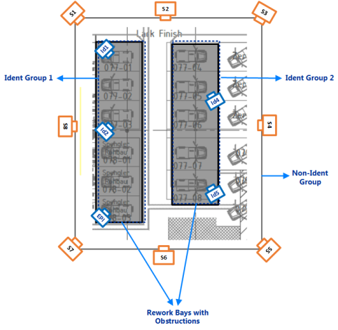
Location Tracking Using a Combination of Ident and non-Ident Sensors

The area is covered completely with non-Ident sensors, which are positioned high-up to provide general tracking capabilities in open areas and aisles. However, the rework bays have heavy obstructions that block these sensors.

Therefore, additional Ident sensors are placed at defined positions inside the bays.

• Sensors Id1, Id2 , and Id3 belong to Ident Group 1.
• Sensors Id4 and Id5 belong to Ident Group 2.
• Non-Ident sensors S1-S8 belong to the non-Ident Group.
• Ident Group 1 and Ident Group 2 are associated with the non-Ident Group, which functions as a Snoop group.

When an Ident sensor receives the strongest signal from the tag (when the car is in a bay), the non‑Ident sensors are ignored. The Ident sensor which is the closest to the tag generates the location.

Note that you could add all Ident sensors to Ident Group 1, but splitting them makes the design clearer.

Custom Sensor Properties

Custom sensor properties provide a method of storing custom parameters for sensors and TDUs beyond the properties provided as standard in the Ubisense dataset, for example to store additional information about sensor locations or unusual configurations. This enables you to maintain all information relevant to your DIMENSION4 sensors in a single location, and with the ability to export this to other sources.

Custom properties are added to the dataset using the ubisense_ls_sensor_properties admin tool, and can be of the type bool, choice, double, int, string, time or timespan. After custom properties have been added, they can be displayed in the Custom sensor properties tab using user-configurable views which can contain a mix of standard and custom properties. You can edit the contents of custom properties (and the standard comment property) in the Custom sensor properties tab.

You can export data for selected sensors from a view, and import custom properties from external sources, in CSV format.

Creating Custom Sensor Properties

Use the ubisense_ls_sensor_properties_admin tool to add custom sensor properties.

You can download this tool using the Application Manager: go to the DOWNLOADABLES tab and open Ubisense > Location system > Administration tools to find it. See the instructions for installing Client Machines for information on downloading tools.

You can add properties of the following types:

• bool
• choice
• double
• int
• string
• time
• timespan

For each custom sensor property you want to add, run the ubisense_ls_sensor_properties_admin tool and specify the property type and description. For example to add a boolean property called new, use the command:

For properties of the type choice, you also specify the list of options. For example, the command:

creates a color property whose values can be black, white or grey.

If you create properties, you will need to restart any instances of LSC before you can see them.

Adding and Editing Views

You can choose properties for display, and the default order in which columns of data are shown, and save them as views. Before you can include custom sensor data in a view, you must have added the necessary properties to your dataset.

To create a view:

1. Click Create new view to display a list of columns available for inclusion in the view.

   The list includes columns for properties supplied with your installation along with columns for any custom properties that have been defined.

2. Give the view a name.

3. Select columns for inclusion and click Add >.

   • Remove columns by selecting them in the selected columns list and clicking < Remove.
   • Select multiple columns by holding down Shift or Ctrl and clicking on them.
4. Select columns in the Selected columns list and use the Move up and Move down buttons to change the order in which they display.
5. When you are happy with your choices, click Save.

Editing a View

You can edit a view by selecting it from the <Select a column view> dropdown and clicking Edit selected view. Add and remove columns and change their display order as described above.

Deleting a View

To delete a view, select it from the <Select a column view> dropdown and click Edit selected view. Select Delete view and click Save.

Viewing Custom Sensor Properties

You choose how you want to display sensor information by choosing a view (see Adding and Editing Views for information on defining the content of a view) and selecting the sensors you are interested in.

To display custom properties for selected sensors:

1. Open the Custom sensor properties tab.

   A list of sensors is shown. This will either be all sensors, or a selection displayed using the Show selected button in this, or another, tab.

2. Choose a view from the <Select a column view> dropdown. The columns for properties included in the view are displayed.

   • You can change the order in which columns are displayed by dragging column headings. Save the new arrangement by clicking Save column order and this will become your default layout when you next select this view. (You can return to the predefined order of columns by clicking Revert column order.)

3. Refine the selection of rows by typing text to search for into <Select matching rows>—the search is case sensitive. All rows with matching text in any of the columns are highlighted.

   • Use the Show groups check box to toggle between a list of sensors and a tree view of sensor groups and sensors.
   • Sort on a column by clicking in its heading.

Editing Custom Properties

Custom properties, and the standard Comment property, are editable.

To edit a custom property, slowly double-click it and type in the field or choose from a dropdown of available values.

You can add identical information for multiple sensors: select the sensors, by holding down Shift or Ctrl and clicking, and then double-click one of your selections or press Enter to open the editor.

 

Importing Custom Sensor Properties

You can import custom property data for sensors from a CSV file. Before you can import custom sensor data, you must have added the necessary properties to your dataset.

The following constraints apply to importing custom sensor properties:

• The import process does not recognize sensors that are not already part of your dataset and does not import data associated with them
• Only custom properties and the standard comment property can have their values updated by the import; other properties are not changed

The CSV file must contain data formatted as comma-separated strings enclosed in quotation marks. The first row of the import file contains the names of the properties to be imported. It is important that the format is correct, as if the import process detects an incorrect format, the import will fail.

You must also take care to ensure that values supplied for custom properties are of the correct type. Otherwise, the import will fail.

To import custom sensor properties:

1. On the Custom sensor properties tab, click Import rows.

2. Type the name of the CSV file or browse to its location.

3. Decide how unknown data is handled:

   • Select Ignore unknown properties to allow the import process to ignore properties that are not configured in your dataset. If this is not selected, and unknown properties are encountered, the import will fail.
   • Select Ignore unknown sensors to allow the import process to skip data for sensors that do not belong to your dataset. If this is not selected, and unknown sensors are encountered, the import will fail.

4. Click Import.

Exporting Custom Sensor Properties

You can export a selection of custom sensor properties to a file in CSV format which can then be used in other applications.

To export custom sensor properties:

1. On the Custom sensor properties tab, display the sensors and properties to be exported. See Viewing Custom Sensor Properties.

2. Click Export rows.
3. Type the name of the file or browse to its location. Select Overwrite existing file if necessary? to replace a file that already exists.

4. Click Export.

Support for DIMENSION4 tags with GPS receivers

Some DIMENSION4 tags contain GPS receivers and can periodically transmit their GPS coordinates via the tag’s onboard 2.4 GHz radio.

From version 3.5 onwards, DIMENSION4 sensors can be configured to receive these transmissions, and the DIMENSION4 support services can be configured to transform the GPS latitude/longitude values into tag position events in the user-defined XYZ coordinate system, so that the GPS readings create tag location events that are sent via the Ubisense OTW protocol or the ISO 24730 protocol exactly as though they were generated from UWB transmissions.

The DIMENSION4 support for GPS tags includes features to support:

• Configuring DIMENSION4 sensors to receive GPS signals from tags via the 2.4G Hz radio
• Creating and configuring GPS reference points using the Background objects screen in Location System Config
• Configuring tag type declarations to make best use of the tags’ onboard tremble switches
• Viewing generated XYZ transformations of the tag GPS positions using the Event review screen in Location System Config
• Tracing the tag GPS protocol and XYZ transformation calculation using the Ubisense tracing features
• Configuring advanced parameters in the GPS processing chain

Configuring DIMENSION4 sensors to receive GPS

To configure a DIMENSION4 sensor to receive GPS messages (and forward them to the calculation services), set the sensor’s radio mode to 56, using the Change sensor parameters / Radio / Mode option, or the equivalent Change all parameters / Sensor / Radio / Mode option shown below:

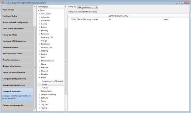
By editing the ‘Sensor / Radio Mode / Value 0’ value on the same screen it is possible to set the receive frequency for the sensor. If the value is left at its default value of zero, the default UbisenseGPS tag frequency (of 2404000 kHz) will be used. Otherwise, the receive frequency in kHz should be used; for example, to use 802.15.4f-2012 channel 15, which is 2401750 kHz, enter 2401750 into the ‘Sensor / Radio Mode / Value 0’ parameter.

Note that, if the sensor supports an external antenna (as in part number D4DETECTOR32IP30), the radio mode does not need to be set in the configuration tool, because the sensor’s internal radio mode will automatically be set to 56 by the sensor’s on-board software. In this case the value of the radio mode in the configuration tool will have no effect (this feature ensures that it is impossible to configure a sensor to transmit 2.4 GHz potentially using a high-gain antenna, which would risk causing RF interference).

Creating and configuring GPS reference points

In order to transform a GPS reading into an XYZ reading it is necessary to define a mapping between the two co-ordinate systems. This is done by creating at least two GPS reference points, which have a position in the XYZ system and also have a latitude, longitude and altitude in the GPS system.

In the ‘Add background objects’ screen of Location System Config, a new ‘reference object’ type ‘GPS reference point’ is now available so that it is possible to drag GPS reference points onto the map.

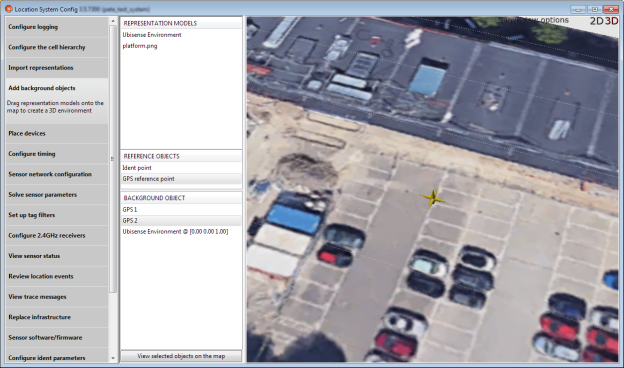
The reference point is shown as a six-pointed gold 3D star. By double-clicking on the reference point, it is possible to configure its name and edit its position.

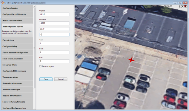
When a reference point has been added, its GPS parameters can be configured in the Change all parameters tab:

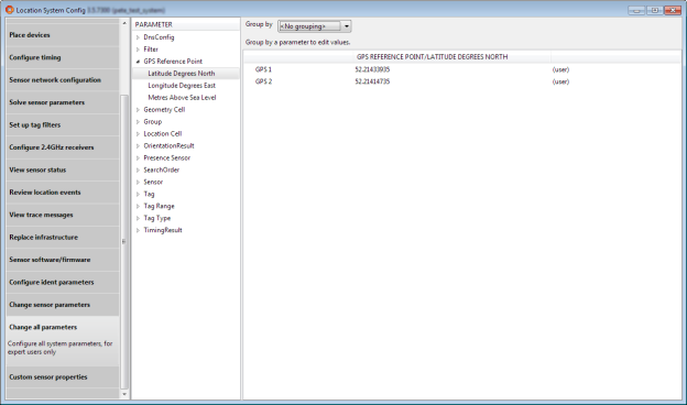
Three parameters are required:

• Latitude Degrees North is the decimal number of degrees north of the equator at the GPS reference point.
• Longitude Degrees East is the decimal number of degrees east of the Prime Meridian at the GPS reference point.
• Metres Above Sea Level is the elevation above sea level of the GPS reference point.

The first two parameters should be entered as accurately as possible. The elevation parameter can be significant in an area of high altitude (e.g. more than 1000 m above sea level) but will have little effect on the result for altitudes much below this.

Configuring tag type declarations

The GPS to XYZ transformation calculation makes use of the tag’s tremble switch as a way of indicating that the tag is moving. But in some cases the tag’s tremble switch will continue to be ‘on’ even when the tag is stationary (for example, if it is attached to a vehicle which will run its engine when stationary, generating enough vibration to activate the tremble switch).

In these cases it is possible to direct the calculation to ignore the tremble switch state by assigning a suitable type to the tag and using the ‘Trembles When Stationary’ attribute of the type to assert that the tag will still tremble even when stationary. This is set by setting the Change all parameters / Tag Type / Trembles When Stationary parameter:

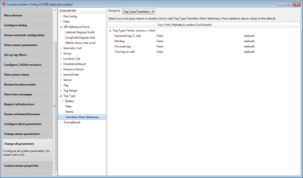
Viewing generated XYZ positions of the tag

When a tag GPS reading is received by a sensor, it is forwarded to the ‘Ubisense / Location system / Location sink’ service in the location cell that owns the sensor. The service will then process the tag’s GPS data, using the GPS reference points that were defined, to transform it into a XYZ data. This XYZ data is then logged to the logging services (if they are running) so that it can be viewed in the Review location events tab in Location System Config.

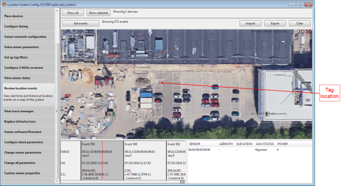
The position of the tag is displayed in grey (here it is in the leftmost column of parking spaces, about 8 m above the two cars).

This ‘raw’ XYZ data is then processed by a median filter in the service. Normally this will result in the generation of another location event, which is a valid tag XYZ reading to be sent out. This event is transmitted to clients using the Ubisense OTW protocol or the ISO 24730 protocol, and another event is also logged for viewing in the event review screen, in this case with the tag’s location shown in red, indicating that this is a valid location:

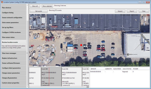
Tracing the tag GPS protocol and calculation

The ls_sink_gps trace stream

The trace stream ‘ls_sink_gps’ will print a trace of processing events from the location sink’s GPS processing. This is not intended to be enabled during GPS operation, but can be a useful aid to understanding the transformation from GPS to XYZ and debugging misconfigurations.

The trace stream messages cover the following events, which occur in sequence in the processing pipeline.

Message reception from the sensor

When the location sink service receives a message from the sensor it prints out its contents

Rejection of duplicate packets

Each sensor listens on two antennas, and multiple sensors may be listening for GPS packets, therefore a packet from an individual tag may result in several GPS packets being received at the location sink. The tag transmits a sequence number in each packet, and to ensure correct processing the location sink will record the sequence number of the last accepted GPS reading and then reject any subsequent packets that have the same sequence number for the given tag. When this happens it will print the message:

Flushing filter state when the tag is moving

If the tag tremble switch is on and either the type of the tag is not set, or the type of the tag is set to a type that is asserted to not tremble when stationary (the default state for a tag type), then the processing will deduce that the tag is moving. The processing maintains some outlier rejection state that assumes that the tag is stationary, so when the tag is moving the state is not valid and must be deleted.

When this happens the location sink will print the message:

Setting up the GPS-XYZ mapping using the reference points

Before processing its first tag event, and every 60 seconds thereafter, the location sink will update its GPS reference points. Two reference points are required in order to create a GPS-XYZ mapping, and if the service cannot find two reference points it will print this message:

If two reference points are retrieved then the service will print out the points that it did get, together with the derived data that is used for building the mapping, as follows: the earth’s radius (the mapping approximates to the Earth’s oblate spheroid geometry by considering it as a sphere whose radius is determined by the latitude and altitude); the distance between the reference points calculated in the XYZ system and in the lat/long system (these values should be close together, and this is a useful check on the configuration); the bearings from one point to another in the XYZ system and in the lat/long system and thus the rotation between the two co-ordinate systems. The sequence of messages looks like this:

Note that the mapping algorithm assumes that the latitude/longitude angle between the two reference points is small, so that the GPS coordinate system near the reference points can be approximated by a Cartesian system in which there is an XY plane which touches the earth’s surface. If this is not possible then it is possible to define multiple mappings, with a different mapping for each Geometry cell. To do this, just place two reference points in each of the Geometry cells that require their own separate mapping – the location sink service will always prefer points that are physically inside its parent Geometry cell.

Rejecting the calculated XYZ if it is too far from the sensor

If the calculated position in the XYZ system is found to be so far from the receiving sensor that it would have been beyond the reception range of the sensor, then the reading is rejected as failing a sanity check. When this happens this message is printed:

Filtering the reading using a median buffer

If the XYZ position has not been rejected by this stage, it is accepted as suitable for insertion into the filtering buffer, and this message is printed:

This value is the same as the raw reading logged in the event review screen.

Extracting a median value for assertion

The outlier rejection filter uses a buffer of readings from which it selects the median value for assertion. The length of the buffer can be specified using the advanced parameters below.

When a suitable median value is selected then a location event is pushed into the clients (via the OTW or ISO 24730 protocols) and the asserted reading is logged in the event review screen, and this message is printed:

ls_sink_gps: injecting <tag id> at <position>

Configuring advanced parameters

There are some advanced parameters available to the location sink. These should not normally require changing but they may be changed by advanced users who have a clear understanding of the implications of their actions.

Parameter	Default value	Purpose
ls_gps_gdop	10.0	Not currently used. Do not modify.
ls_gps_stderr	10.0	The value to be used as the error estimate in meters when sending location events using the OTW protocol
ls_gps_range	300.0	The expected maximum range in meters at which a sensor can pick up a GPS tag transmission
ls_gps_buf_min	3	The minimum length of the median buffer (defaults to 3, must be >1, and will be increased to the nearest odd number)
ls_gps_buf_max	11	The maximum length of the median buffer (defaults to 11, must be < 101, and will be increased to the nearest odd number)

Configuring Battery Usage Monitoring

To enable the battery usage monitoring for a particular tag, you need to assign a tag type to the tag and that tag type must be configured with appropriate battery capacity information. This will, for example, allow the battery usage status to be displayed on a web browser by the tag operations screen in Ubisense SmartSpace Visibility.